This site contains links to data sets from the SandyDuck nearshore two-dimensional array of Sonar altimeters (S), Pressure gages (P), bi-directional current meters (UV), and Thermistors (T, colocated with pressure sensors) deployed from near the shoreline to 5-m water depth along about 200 m of the coast during August-December 1997.
The schematic shows the sensor locations (and approximate water depths) in the Field Research Facility (FRF) coordinate system.
-
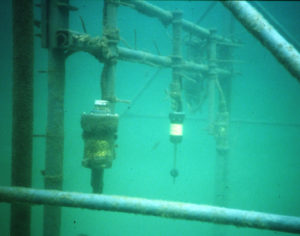
- A close up view of a SPUVT frame under water a few days after being deployed. The bio-fouled cylindrical instrument on the left (with white cap on top and yellow ring) is a pressure gage. The clean sensor to the right (also has a bright yellow ring, with black 2 cm diamter sphere below) is an electromagnetic current meter. Biofouling results in slow degradation of data from electromagnetic current meters, requiring weekly cleaning and recalibration of offsets. (Photographs courtesy of W. Birkemeier, FRF.)

-
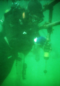
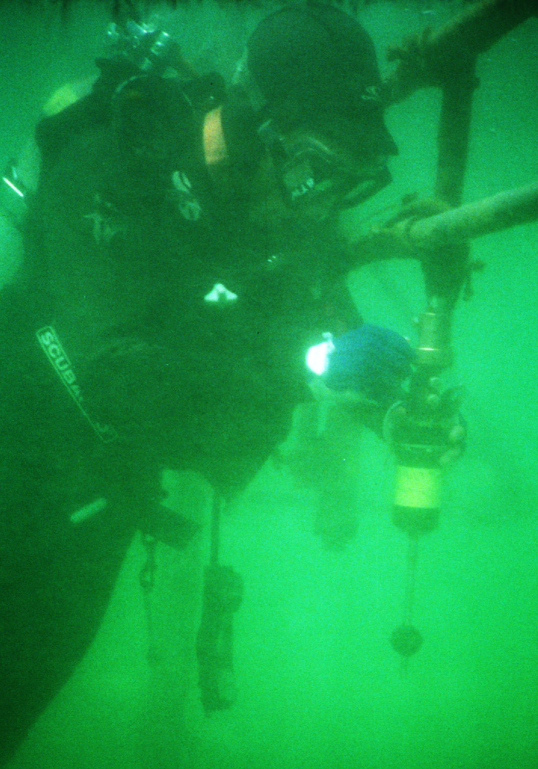
- Scripps engineer Brian Woodward has cleaned the electromagnetic current meter and is rotating it 180-degrees as part of the in-field recalibration process. All 40 current meters were cleaned and recalibrated approximately every 7-10 days to obtain mean currents with +/- 5 cm/s accuracy. (Photographs courtesy of W. Birkemeier, FRF.)
-
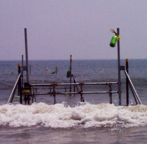
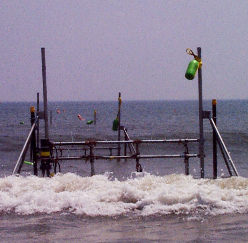
- A SPUVT frame near the shoreline at low tide. Mounted on the horizontal cross bars (from left to right) are an electronics package (yellow ring, 4 cables), a sonar altimeter, a Marsh McBirney electomagnetic current meter, and under water on the right hand side is a pressure gage. The cross bars are adjustable vertically to maintain the current meter about 50 cm over the evolving seafloor. Thirty-six frames were deployed in a two-dimensional array. (Photographs courtesy of W. Birkemeier, FRF.)
Examples of Data from the SPUVT Array
Example 1:
Long Time Series of 5-M Depth SandyDuck Observations
The 2D array of SandyDuck sensors acquired observations of waves, currents, and seafloor location nearly continuously from 1 Aug thru 3 Dec 1997. The figure shows 3-hr mean values of significant wave height (Hsig, top panel), alongshore current (V, second-from-top panel), and cross-shore current (U, third-from-top panel) versus time. Positive V is upcoast (approximately northward) flow, and positive U is onshore flow. These observations were made in approximately 5-m water depth at the offshore edge of the cross-shore transect in the center of the array (cross-shore coordinate = 385 m, longshore coordinate = 827.5 m (see the array plan). The bottom panel shows the approximate cross-shore location of the crest of the sand bar as a funtion of time (determined by a combination of daily-weekly amphibious vehicle surveys and 3-hourly sonar altimeter estimates of seafloor location.
Example 1. LONG TIME SERIES OF 5-M DEPTH SANDYDUCK OBSERVATIONS
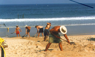 From water’s edge to dry beach, Bill Boyd (red trunks, straw hat), Steve Elgar (scrawny guy with white hat), Jerry ‘DW’ Wanetick (dark hat) , Kimball Millikan (no hat), and Kent Smith (buff tan guy with white hat) digging a trench across the beach at Duck to bury a cable connecting offshore instruments to data acquisition computers located in a trailer at the FRF. This is the only known photograph of Bill Boyd (red trunks) with a shovel, and clearly he has not learned how to operate it. Guza may have been taking a nap. Just offshore of the white foam (broken wave) is a SPUVT frame, and at the water’s edge just seaward of the trenching crew (on the left side of the photograph) is a frame with acoustic doppler currents meters in a pilot test performed by Britt Raubenhiemr to observe swash velocities. (Photograph courtesy of W. Birkemeier, FRF.)
Example 2:
Observations from One 3-hr Data Set
The SandyDuck observations were acquired nearly continuously in 3-hr long pieces, synchronized with the FRF data collection. Means (and variances) of bottom pressure (eg, water depth), wave height and direction, cross- and alongshore velocity, and seafloor location were calculated for each 3-hr run. The arrows in the top panel of the figure point in the direction of wave propagation and have length proportional to the variance of sea-surface elevation in the frequency (f) band 0.07 < f < 0.25 Hz. The arrows get shorter as waves break in the surfzone (cross-shore coordinate less than approximately 200 m). The offshore significant wave height was about 2 m. The waves shoal over the nearshore bathymtery (a map based on altimeter estimates for this 3 hour run is shown in the center panel), break in shallow water, and drive nearshore circulation (lower panel, the arrows point in the direction of the near-bottom currents, with length proportonal to current speed.) In this energetic wave example, surfzone currents were as great as 89 cm/s. The base of each arrow corresponds to an instrument location.
Example 2. OBSERVATIONS FOR ONE 3-hr DATA SET
Example 3:
48-hr Sequence of Mean Currents
A time sequence of 3-hr mean currents showing the evolution of nearshore circulation from weak northerly and offshore flows to strong southerly flows (arrows pointing towards the bottom of the page) as the wind increased from calm to more than 25 knots from the northeast. Each arrow points in the direction of the flow, with length proportional to the current speed. A 30 cm/s scale is shown in the upper left. The numbers at the base of each arrow are the sensor identity. The date and time of each set of mean flows is listed at the top in the format MMDDHHHH, where MM=month, DD=day, HHHH = hour (EST) of the start of the 3-hr record.
Example 3. 48-hr SEQUENCE OF MEAN CURRENTS
Publications
For more information contact Steve Elgar, elgar@whoi.edu or Bob Guza, rtg@coast.ucsd.edu. Conducted Aug-Dec 1997 in Duck, NC at the Field Research Facility.
Download Data
Please fill out the below form to access data files.
"*" indicates required fields
Funded by