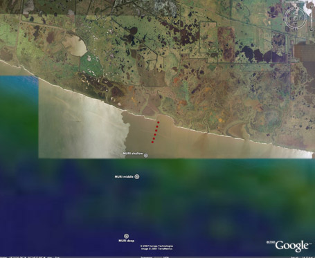
Aerial view of the Louisiana coast and the sensors (red symbols) shown in the above panel, as well as the 3 tripods deployed by the MURI team (white symbols).
To develop, test, and improve models for the dissipation of ocean surface-gravity waves propagating over a muddy seafloor in shallow water, observations of waves were collected for 24 days in March and April 2007 along the transect shown in Figure 1.
The seafloor was covered with a 30-cm thick layer of yogurt-like mud (density about 1.6 g/l [G. Kineke and S. Bentley]) that caused significant dissipation of the wave field, as shown in Figure 2. For example, during a small storm (waves were 1 m high in 5-m water depth) on day 22, there was a 70% reduction in energy flux (a quantity that is conserved in the absence of dissipation) as waves propagated 1.8 km between about 5 and 2 m depth (Figure 2, compare the black curve (most offshore sensor in Figure 1) with the red curve (most onshore sensor in Figure 1)).
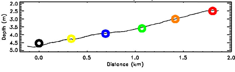
Figure 1. Depth (curve) of the muddy seafloor versus distance from the most offshore sensor measured during a shipboard acoustic survey (provided by G. Kineke). Symbols are colocated pressure gages and current meters.
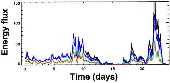
Figure 2. Energy flux versus time. Thick black and blue curves are the energy fluxes (m3/s) observed in approximately 5- and 4-m water depths (same colors as symbols in Figure 1). The red curve is the energy flux observed in approximately 2-m depth (red symbol in Figure 1), 1.8 and 1.1 km onshore of the black and blue curves, respectively. Energy fluxes at the shallowest sensor (red symbol in Figure 1) predicted by a nonlinear Boussinesq wave model that includes an empirical mud-induced dissipation function are shown by the thin turquoise (initialized 1.8 km away) and green (initialized 1.1 km away) curves. If the model were perfect, the thin turquoise and green curves would overlay the red curve.
An estimate of the frequency dependence of the mud-induced dissipation was obtained by comparing the observations with predictions from a nondissipative nonlinear Boussinesq wave model. The model was initialized with observations at each sensor location, and integrated to the next sensor shoreward. Differences between model predictions and observations at the shoreward sensor are attributed to dissipation. A nonlinear wave model is required because in these water depths nonlinear interactions can result in large transfers of energy between waves with different frequencies that otherwise might be incorrectly attributed to dissipation. By reinitializing the model at each sensor location, accumulation of model errors is reduced.
This empirical dissipation function was used in the nonlinear Boussinesq model to simulate the wave field. The dissipative Boussinesq wave model was initialized with observations at the sensors located 1.8 (black symbol in Figure 1) and 1.1 (blue symbol in Figure 1) km offshore of the shallowest sensor (red symbol in Figure 1), and integrated shoreward. The model predictions of the overall energy fluxes are similar to those observed at the shallow sensor (compare thin turquoise and green curves with the red curve in Figure 2).
Preliminary results can be found in “Wave Dissipation by Muddy Seafloors,” by Elgar and Raubenheimer (in press, GRL).
Data Download
Please fill out the below form to access data files.
"*" indicates required fields
Funded by